Day 5: Linear, Ridge, and Logistic Regression & Train-Test Split
Agenda
- 3:45-4:00pm: Debrief at tables
- 4:00-4:20pm: Ridge Regression
- 4:20-5:10pm: Classification and train/test split
- 5:10-5:25pm: Logistic Regression Primer
Debrief on the last assignment (15 minutes)
What were your major conclusions regarding the models used in the EchoMinds app? As a reminder, here were the prompts.
- Are these two datasets useful for evaluating the EchoMinds app? How do they fit with app’s value proposition? How are they misaligned?
- How did the models work when you tried your own questions? Were you able to fool the models by choosing particular wordings for your questions?
- Based on your analysis, what tasks could the EchoMinds app do right now and what conditions (or tasks) would be beyond its capabilities?
Ridge Regression Math (20 minutes)
You’ll do some more on ridge regression in the assignment, including an exploration of why it’s useful. In class, we’re going to go over the math of ridge regression (which will also be an exercise on your assignment).
One way to mitigate the problem of having two little data or having features that are linear combinations of each other is to modify the linear regression problem to prefer solutions that have small weights. We do this by penalizing the sum of the squares of the weights themselves. This is called ridge regression (or Tikhonov regularization). Below, we show the original version of ordinary least squares along with ridge regression.
Ordinary least squares:
\[\begin{align*} \mathbf{w^\star} &= \argmin_\mathbf{w} \sum_{i=1}^n \left ( \mathbf{w}^\top \mathbf{x_i} - y_i \right)^2 \\ &= \argmin_\mathbf{w} \left ( \mathbf{X}\mathbf{w} - \mathbf{y} \right)^\top \left ( \mathbf{X}\mathbf{w} - \mathbf{y} \right) \end{align*}\]Formula for the optimal weights in linear regression:
\[\begin{align*} \mathbf{w^\star} = \left ( \mathbf{X}^\top \mathbf{X} \right)^{-1} \mathbf{X}^\top \mathbf{y} \end{align*}\]Ridge regression (note that $\lambda$ is a non-negative parameter that controls how much the algorithm cares about fitting the data and how much it cares about having small weights):
\[\begin{align*} \mathbf{w^\star} &= \argmin_\mathbf{w} \sum_{i=1}^n \left ( \mathbf{w}^\top \mathbf{x_i} - y_i \right)^2 + \lambda\sum_{i=1}^d w_i^2 \\ &= \argmin_\mathbf{w} \left ( \mathbf{X}\mathbf{w} - \mathbf{y} \right)^\top \left ( \mathbf{X}\mathbf{w} - \mathbf{y} \right) + \lambda \mathbf{w}^\top \mathbf{w} \end{align*}\]The penalty term may seem a little arbitrary, but it can be motivated on a conceptual level pretty easily. The basic idea is that in the absence of sufficient training data to suggest otherwise, we should try to make the weights small. Small weights have the property that changes to the input result in minor changes to our predictions, which is a good default behavior.
Derive an expression to compute the optimal weights, $\mathbf{w^\star}$, to the ridge regression problem.
Classification and Train/Test Split in scikit-learn (50 minutes)
Overfitting our model to our data can lead to diminished results when we apply our model to a new set of data. One of the ways we try to avoid overfitting is by splitting our data into a training and testing set. (In the future, we will talk about another split of the training data called cross-validation, but for now, we won’t worry about that.)
Scikit-learn is a common python library for classic machine learning.
We are going to do a guided tour of this Colab notebook on classification
Logistic Regression Primer (15 minutes)
We’ve met the idea of classification. Logistic regression is one algorithm for binary classification. It builds nicely on linear regression and feeds nicely into neural networks (which we will explore soon).
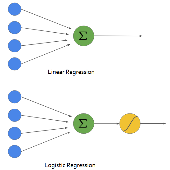
Graphical representation of both linear and logistic regression. The key difference is the application of the squashing function shown in yellow. Original Source - Towards Data Science
If we finish this early, let’s move onto the assignment where you’ll be meeting loss functions for binary classification.