Assignment 2

Learning Objectives

Learning Objectives

• Learn linear regression from three angles:
  • “top-down” (big picture, visual)
  • “bottom-up” (mathematical derivation)
  • computational (implementing in python)
• build python skills of dealing with data and writing functions

Supervised Learning Problem Setup

Suppose you are given a training set of data points, $(\mathbf{x_1}, y_1), (\mathbf{x}_2, y_2), \ldots, (\mathbf{x}_n, y_n)$ where each $\mathbf{x_i}$ represents an element of an input space (e.g., a d-dimensional feature vector) and each $y_i$ represents an element of an output space (e.g., a scalar target value). We will consider $\mathbf{x_i}$ to be a row vector of size 1 x d, representing each of the feature values for one sample/exemplar, as this will make our lives easier when we get more data points. In the supervised learning setting, your goal is to determine a function $\hat{f}$ that maps from the input space to the output space. For example, if we provide an input $\mathbf{x}$ to $\hat{f}$ it would generate the predicted output $\hat{y} = \hat{f}(\mathbf{x})$.

We typically also assume that there is some loss function, $\ell$, that determines the amount of loss that a particular prediction $\hat{y_i}$ incurs due to a mismatch with the actual output $y_i$. We can define the best possible model, $\hat{f}^\star$ as the one that minimizes these losses over the training set. This notion can be expressed with the following equation (note: that $\argmin$ in the equation below just means the value that minimizes the expression inside of the $\argmin$, e.g., $\argmin_{x} (x - 2)^2 = 2$, whereas $\min_{x} (x-2)^2 = 0$).

\[\begin{aligned} \hat{f}^\star &= \argmin_{\hat{f}} \sum_{i=1}^n \ell \left ( \hat{f}(\mathbf{x_i}), y_i \right ) \end{aligned}\]

Linear Regression from the Top-Down

Motivation: Why Learn About Linear Regression?

Before we jump into the what of linear regression, let’s spend a little bit of time talking about the why of linear regression. As you’ll soon see, linear regression is among the simplest (perhaps the simplest) machine learning algorithm. It has many limitations, which you’ll also see, but also a of ton strengths. First, it is a great place to start when learning about machine learning since the algorithm can be understood and implemented using a relatively small number of mathematical ideas (you’ll be reviewing these ideas later in this assignment). In terms of the algorithm itself, it has the following very nice properties.

• Transparent: it’s pretty easy to examine the model and understand how it arrives at its predictions.
• Computationally tractable: models can be trained efficiently on datasets with large numbers of features and data points.
• Easy to implement: linear regression can be implemented using a number of different algorithms (e.g., gradient descent, closed-form solution). Even if the algorithm is not built into your favorite numerical computation library, the algorithm can be implemented in only a couple of lines of code.

For linear regression our input data, $\mathbf{x_i}$, are d-dimensional row vectors (each entry of these vectors can be thought of as a feature), our output data, $y_i$, are scalars, and our prediction functions, $\hat{f}$, are all of the form $\hat{f}(\mathbf{x}) =\mathbf{x} \cdot \mathbf{w} = \mathbf{x} \mathbf{w} = \sum_{i=1}^d x_i w_i$ for some vector of weights $\mathbf{w}$ (you could think of $\hat{f}$ as also taking $\mathbf{w}$ as an input, e.g., writing $\hat{f}(\mathbf{x}, \mathbf{w}$). Most of the time we’ll leave $\mathbf{w}$ as an implicit input: writing $\hat{f}(\mathbf{x})$).

In the function, $\hat{f}$, the elements of the vector $\mathbf{w}$ represent weights that multiply various dimensions (features) of the input. For instance, if an element of $\mathbf{w}$ is high, that means that as the corresponding element of $\mathbf{x}$ increases, the prediction that $\hat{f}$ generates would also increase (you may want to mentally think through other cases, e.g., what would happen is the element of $\mathbf{x}$ decreases, or what would happen if the entry of $\mathbf{w}$ was large and negative). The products of the weights and the features are then summed to arrive at an overall prediction.

Given this model, we can now define our very first machine learning algorithm: ordinary least squares (OLS)! In the ordinary least squares algorithm, we use our training set to select the $\mathbf{w}$ that minimizes the sum of squared differences between the model’s predictions and the training outputs. Thinking back to the supervised learning problem setup, this corresponds to choosing $\ell(y, \hat{y}) = (y - \hat{y})^2$. Therefore, the OLS algorithm will use the training data to select the optimal value of $\mathbf{w}$ (called $\mathbf{w}^\star$), which minimizes the sum of squared differences between the model’s predictions and the training outputs.

\[\begin{aligned} \mathbf{w}^\star &= \argmin_{\mathbf{w}} \sum_{i=1}^n \ell \left ( \hat{f}(\mathbf{x_i}, \mathbf{w}) , y_i \right) \\ &= \argmin_{\mathbf{w}} \sum_{i=1}^n \left ( \hat{f}(\mathbf{x_i}, \mathbf{w}) - y_i \right)^2 \\ &= \argmin_{\mathbf{w}} \sum_{i=1}^n \left ( \mathbf{x_i} \mathbf{w} - y_i \right)^2 \end{aligned}\]

Notice

Digesting mathematical equations like this can be daunting, but your understanding will be increased by unpacking them carefully. Make sure you understand what was substituted and why in each of these lines. Make sure you understand what each symbol represents. If you are confused, ask for help (e.g., post on Slack).

Below, we will talk about how to find $\mathbf{w}^\star$, for now we’ll just assume we have it. With $\mathbf{w}^\star$, we can predict a value for a new input sample, $\mathbf{x_i}$, by predicting the corresponding (unknown) output, $y_i$, as $\hat{y_i} = \mathbf{x_i} \mathbf{w^\star}$. Because $\mathbf{x_i}$ is a row vector, this is equivalent to the dot product. At this point, we have used the training data to learn how to make predictions about unseen data, which is the hallmark of supervised machine learning!

Exercise 1

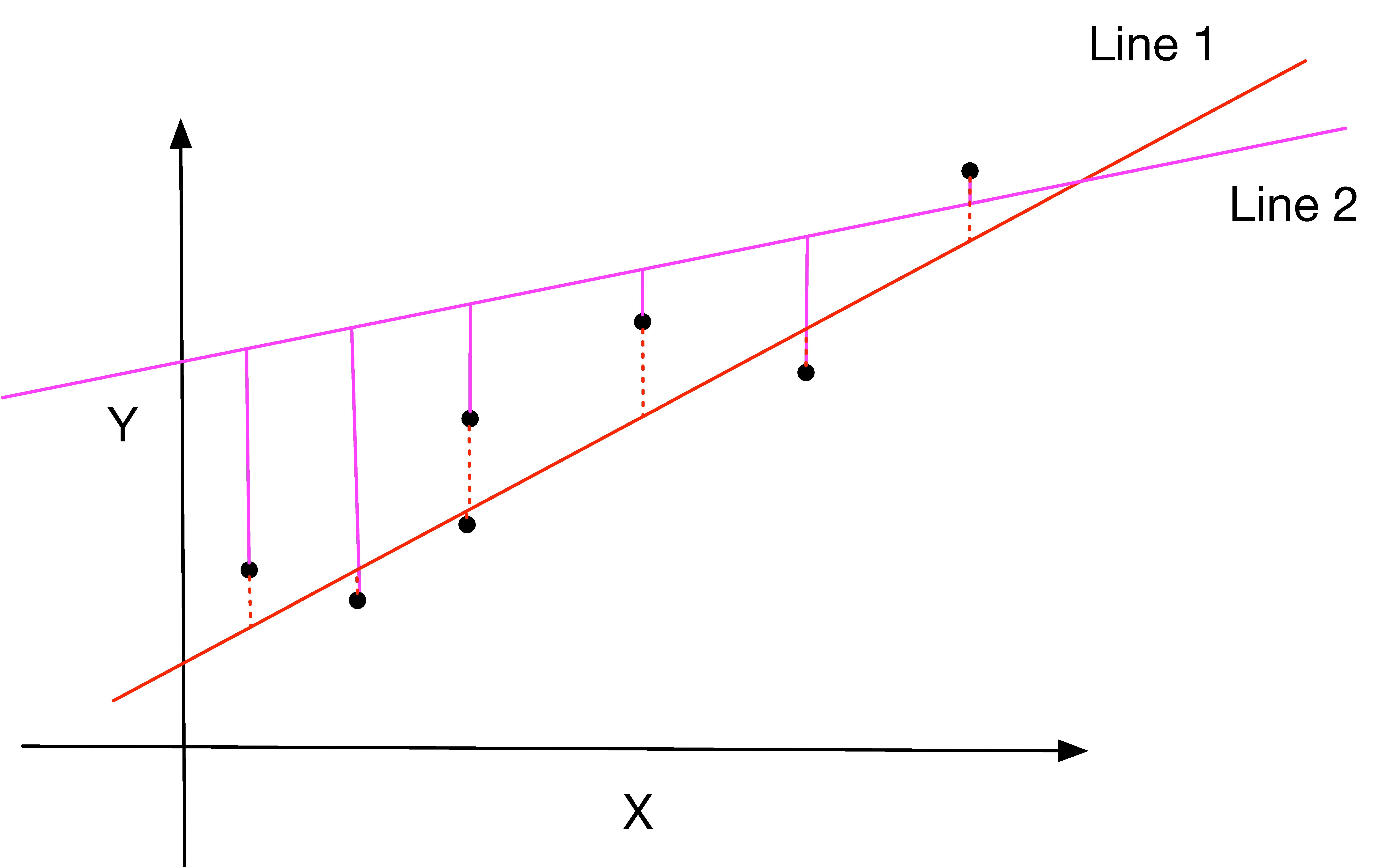
Draw a scatter plot in 2D (the x-axis is the independent variable and the y-axis is the dependent variable). In other words, draw five or so data points, placed wherever you like. Next, draw a potential line of best fit, a straight line that is as close to your data points. On the plot mark the vertical differences between the data points and the line (these differences are called the residuals). Draw a second potential line of best fit and mark the residuals. From the point of view of ordinary least-squares, which of these lines is better (i.e. has the smallest residuals)?

Solution

The red line (line 1) would be better since the residuals are generally smaller. Line 2 also has several large residuals, which when squared will cause a large penalty for line 2.

Getting a Feel for Linear Regression

In this class we’ll be learning about algorithms using both a top-down and a bottom-up approach. By bottom-up we mean applying various mathematical rules to derive a solution to a problem and only then trying to understand how to apply it and how it well it might work for various problems. By top-down we mean starting by applying the algorithm to various problems and through these applications gaining a sense of the algorithm’s properties. We’ll start our investigation of linear regression using a top-down approach.

Linear Regression with One Input Variable: Line of Best Fit

If any of what we’ve said so far sounds familiar, it is likely because you have seen the idea of a line of best fit in some previous class. To understand more intuitively what the OLS algorithm is doing, we want you to investigate its behavior when there is a single input variable (i.e., you are computing a line of best fit).

Exercise 2

Use the line of best fit online app to create some datasets, guess the line of best fit, and then compare the results to the OLS solution (line of best fit).

Part A

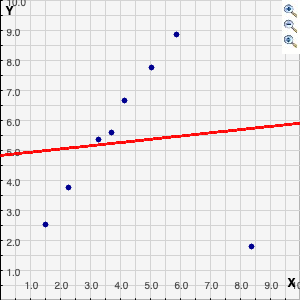
Examine the role that outliers play in determining the line of best fit. Does OLS seem sensitive or insensitive to the presence of outliers in the data?

Solution

OLS is very sensitive to outliers. A single outlier can change the slope of the line of best fit dramatically. Here is an example of this phenomenon.

Part B

Were there any times when the line of best fit didn’t seem to really be “best” (e.g., it didn’t seem to capture the trends in the data)?

Solution

This could happen for many reasons. If the dataset is pieceweise linear (e.g., composed of multiple line segments), if it has some other non-linear form (e.g., if it is quadratic), or if there are outliers.

Linear Regression from the Bottom-Up

Now that we’ve built a little intuition on linear regression, we’ll be diving into the mathematics of how to find the vector $\mathbf{w}^\star$ that best fits a particular training set. The outline of the steps we are going to take to learn this are:

1. Solve the special case of linear regression with a single input ($d=1$, meaning a 1-dimensional feature vector).
2. Learn some mathematical tricks for manipulating matrices and vectors and computing gradients of functions involving matrices and vectors (these will be useful for solving the general case of linear regression).
3. Solve the general case of linear regression (where $d$ can be any positive, integer value).

Linear regression with one variable

Exercise 3

Part A

Given a dataset $(x_1, y_1), (x_2, y_2), \ldots, (x_n, y_n)$ (where each $x_i$ and each $y_i$ is a scalar) and a potential value of $w$ (note that $w$ is a scalar in the case where $d=1$), write an expression for the sum of squared errors between the model predictions, $\hat{f}$, and the targets, $y_i$. Note: In contrast to the line of best fit we saw above, here we are not computing a y-intercept (so we are effectively forcing the y-intercept to be $0$). This choice may result in a worse fit, but it is easier to work out and helps build mathematical intuition.

Solution

\[\text{Sum of Squared Errors} = e(w) = \sum_{i=1}^n \left ( x_i w - y_i \right)^2~~ \\ \text{ (note: we define error $e(w)$ for convenience)}\]

Part B

Compute the derivative of the expression for the sum of squared errors from part (a).

Solution

\[\begin{aligned} \frac{de}{dw} & = \sum_{i=1}^n 2 \left ( x_i w - y_i \right)x_i \\ &= w \sum_{i=1}^n 2 x_i^2 - \sum_{i=1}^n 2 x_i y_i \end{aligned}\]

Part C

Set the derivative to 0, and solve for $w^\star$. $w^\star$ corresponds to a critical point of your sum of squared errors function. Is this critical point a minimum, maximum, or neither? (here is a refresher on classifying critical points).

Solution

\[\begin{aligned} \frac{de}{dw} &= 0 \\ &= w^\star \sum_{i=1}^n 2 x_i^2 - \sum_{i=1}^n 2 x_i y_i \\ \sum_{i=1}^n 2 x_i y_i &= w^\star \sum_{i=1}^n 2 x_i^2 \\ w^\star &=\frac{\sum_{i=1}^n x_i y_i}{\sum_{i=1}^n x_i^2} \end{aligned}\]

If we take the second derivative of $e(w)$ we get:

\[\begin{aligned} \frac{d^2e}{dw^2} &= \sum_{i=1}^n 2x_i^2 \enspace . \end{aligned}\]

We can see from the form of the second derivative that it is always non-negative, and therefore the critical point at $w^\star$ corresponds to a minimum.

Reminder of mathematical ideas

In a previous assignment, we asked you to solidify your knowledge of three different mathematical concepts. The box below summarizes what you were supposed to learn and provides the resources we provided to help you.

External Resources

• Vector-vector multiplication: Section 2.1 of Zico Kolter’s Linear Algebra Review and Reference

• Matrix-vector multiplication
  • Section 2.2 of Zico Kolter’s Linear Algebra Review and Reference
  • The first bits of the Khan academy video on Linear Transformations
• Partial derivatives and gradients
  • Khan Academy videos on partial derivatives: intro, graphical understanding, and formal definition
  • Khan Academy video on Gradient

Building our bag of mathematical tricks

The derivation of linear regression for the single variable case made use of your background from single variable calculus, and you used some rules for manipulating such functions. When approaching linear regression with multiple variables, you have two choices.

1. You can apply the same bag of tricks you used for the single variable problem and only at the end convert things (necessarily) to a multivariable representation.
2. You can approach the whole problem from a multivariable perspective.

This second approach requires that you learn some additional mathematical tricks, but once you learn these tricks, the derivation of linear regression is very straightforward. The secondary benefit of this approach is that the new mathematical tricks you learn will apply to all sorts of other problems.

Exercise 4

A quadratic form can be expressed in matrix-vector form as $\mathbf{x}^\top \mathbf{A} \mathbf{x}$. Written this way, it looks very mysterious, but in this exercise you’ll build some intuition about what the expression represents. Further, it turns out that expressions like this show up in all sorts of places in machine learning. To get a better understanding of what a quadratic form is (we’ll see what it’s good for later), watch this Khan Academy video.

After you’ve watched the Khan academy video, answer these questions.

Note: This $\mathbf{x}$ is a generic column vector, not the $\mathbf{x_i}$ sample vector of features that we were talking about above. We are using the generic $\mathbf{x}$ here to align with the way most resources explain this form.

Part A

Multiply out the expression \(\begin{bmatrix} x_1 \\ x_2 \\ x_3 \end{bmatrix}^\top \begin{bmatrix} a_{1,1} & a_{1,2} & a_{1,3} \\ a_{2,1} & a_{2,2} & a_{2,3} \\ a_{3,1} & a_{3,2} & a_{3,3} \end{bmatrix}\begin{bmatrix} x_1 \\ x_2 \\ x_3 \end{bmatrix}\).

Solution

\[\begin{aligned} \begin{bmatrix} x_1 \\ x_2 \\ x_3 \end{bmatrix}^\top \begin{bmatrix} a_{1,1} & a_{1,2} & a_{1,3} \\ a_{2,1} & a_{2,2} & a_{2,3} \\ a_{3,1} & a_{3,2} & a_{3,3} \end{bmatrix}\begin{bmatrix} x_1 \\ x_2 \\ x_3 \end{bmatrix} &= \begin{bmatrix} x_1 \\ x_2 \\ x_3 \end{bmatrix}^\top \begin{bmatrix} a_{1,1} x_1 + a_{1,2} x_2 + a_{1,3} x_3 \\ a_{2,1} x_1 + a_{2,2} x_2 + a_{2,3} x_3 \\ a_{3,1} x_1 + a_{3,2} x_2 + a_{3,3} x_3 \end{bmatrix} \\ &= a_{1,1} x_1^2 + a_{1,2}x_1x_2 + a_{1,3} x_1 x_3 + a_{2,1}x_1 x_2 + a_{2,2} x_2^2 \nonumber \\ &+ a_{2,3} x_2 x_3 + a_{3,1} x_3 x_1 + a_{3,2} x_3 x_2 + a_{3,3} x_3^2 \end{aligned}\]

Part B

Complete the following expression labeled (i) by filling in the part on the righthand side inside the nested summation.

\(\begin{bmatrix} x_1 \\ x_2 \\ \vdots \\ x_d \end{bmatrix}^\top\begin{bmatrix} a_{1,1} & a_{1,2} & \ldots & a_{1,d} \\ a_{2,1} & a_{2,2} & \ldots & a_{2,d} \\ \vdots & \vdots & \ddots & \vdots \\ a_{d,1} & a_{d,2} & \ldots & a_{d,d} \end{bmatrix}\begin{bmatrix} x_1 \\ x_2 \\ \vdots \\ x_d \end{bmatrix} = \sum_{i=1}^d \sum_{j=1}^d \left (\text{your answer here} \right)\)

Solution

\[\begin{aligned} \begin{bmatrix} x_1 \\ x_2 \\ \vdots \\ x_d \end{bmatrix}^\top \begin{bmatrix} a_{1,1} & a_{1,2} & \ldots & a_{1,d} \\ a_{2,1} & a_{2,2} & \ldots & a_{2,d} \\ \vdots & \vdots & \ddots & \vdots \\ a_{d,1} & a_{d,2} & \ldots & a_{d,d} \end{bmatrix}\begin{bmatrix} x_1 \\ x_2 \\ \vdots \\ x_d \end{bmatrix} &= \begin{bmatrix} x_1 \\ x_2 \\ \vdots \\ x_d \end{bmatrix}^\top \begin{bmatrix} \sum_{j=1}^d a_{1,j} x_j \\ \sum_{j=1}^d a_{2,j} x_j \\ \vdots \\ \sum_{j=1}^d a_{d,j} x_j \end{bmatrix} \\ &= \sum_{i=1}^d \sum_{j=1}^d a_{i,j} x_i x_j \end{aligned}\]

Exercise 5

Matrix multiplication distributes over addition. That is, $(\mathbf{A} + \mathbf{B}) (\mathbf{C} + \mathbf{D}) = \mathbf{A}\mathbf{C} + \mathbf{A}\mathbf{D} + \mathbf{B} \mathbf{C} + \mathbf{B} \mathbf{D}$. Use this fact coupled with the fact that $\left(\mathbf{A} \mathbf{B} \right)^\top = \mathbf{B}^\top \mathbf{A}^\top$ to expand out the following expression.

\[\left ( \mathbf{A} \mathbf{x} + \mathbf{y} \right )^\top \left (\mathbf{v} + \mathbf{u} \right)\]

Solution

\[\left ( \mathbf{A} \mathbf{x} + \mathbf{y} \right )^\top \left (\mathbf{v} + \mathbf{u} \right) = \mathbf{x}^\top \mathbf{A}^\top \mathbf{v} + \mathbf{x}^\top \mathbf{A}^\top \mathbf{u} + \mathbf{y}^\top \mathbf{v} + \mathbf{y}^\top \mathbf{u}\]

Exercise 6

Part A

Using the definition of the gradient, show that $\nabla \mathbf{c}^\top \mathbf{x} = \mathbf{c}$ where the gradient is taken with respect to $\mathbf{x}$ and $\mathbf{c}$ is a vector of constants.

If you want a hint, but not the full solution, you can click on the “solution” for the hint section below. Note: to read the hints, you need to have the version of the assignment open that has the Show Solutions button.

Solution

\[\begin{aligned} \mathbf{c}^\top \mathbf{x} &= \sum_{j=1}^d c_j x_j \\ \frac{\partial}{\partial x_i} \sum_{j=1}^d c_j x_j &= c_i \\ \nabla \mathbf{c}^\top \mathbf{x} &= \mathbf{c} \end{aligned}\]

Part A hint

Solution

Start by writing out the multiplication in the summation form. Then think about the partial derivative with respect to some $i^{th}$ element of $\mathbf{x}$.

Part B

Using the definition of the gradient, show that the $\nabla \mathbf{x}^\top \mathbf{A} \mathbf{x} = 2 \mathbf{A} \mathbf{x}$ where the gradient is taken with respect to $\mathbf{x}$, and $\mathbf{A}$ is a symmetric $dxd$ matrix of constants.

Hint: utilize the fact that $\mathbf{x}^\top \mathbf{A} \mathbf{x} = \sum_{i=1}^d\sum_{j=1}^d x_i x_j a_{i, j}$.

If you are stuck and want a hint, but not the full solution, you can click on the “solution” for the hint section below.

Solution

\[\begin{aligned} \mathbf{x}^\top \mathbf{A} \mathbf{x} =& \sum_{i=1}^d\sum_{j=1}^d x_i x_j a_{i, j} &\nonumber \\ \frac{\partial \mathbf{x}^\top \mathbf{A} \mathbf{x}}{\partial x_k} &= \sum_{i=1}^d\sum_{j=1}^d a_{i,j} \left ( \frac{\partial{x_i }}{\partial x_k} x_j + x_i \frac{\partial{x_j}}{\partial x_k} \right) \text{ } \text{apply the product rule} \nonumber \\ &= \sum_{i=1}^d\sum_{j=1}^d a_{i,j} \frac{\partial{x_i }}{\partial x_k} x_j + \sum_{i=1}^d\sum_{j=1}^d a_{i,j} x_i \frac{\partial{x_j}}{\partial x_k} \text{ }\text{ split into two summations} \nonumber \\ &= \sum_{j=1}^d a_{k,j} x_j + \sum_{i=1}^d a_{i,k} x_i \text{ }\text{take partial derivatives, many terms are 0} \nonumber \\ &= \sum_{j=1}^d a_{k,j} x_j + \sum_{i=1}^d a_{k,i} x_i \text{ } \text{ since $\mathbf{A}$ is symmetric, $a_{i,j} = a_{j,i}$} \nonumber \\ &= 2 \sum_{j =1}^d a_{k,j} x_j \text{ } \text{the two summations are the same} \nonumber \\ &= 2 \mathbf{row}_k^\top \mathbf{x} \text{ } \text{this is the dot product between $\mathbf{x}$ and the $k$th row of $\mathbf{A}$} \nonumber \\ \nabla \mathbf{x}^\top \mathbf{A} \mathbf{x} &= 2 \mathbf{A}\mathbf{x} \text{ } \text{stacking up the partials gives this form} \nonumber \end{aligned}\]

Part B hint

Solution

You can use the concepts in the first part of this exercise to expand things out to a summation. After a little work, you should reach something that looks like: \(\frac{\partial \mathbf{x}^\top \mathbf{A} \mathbf{x}}{\partial x_k} = \sum_{i=1}^d\sum_{j=1}^d a_{i,j} \frac{\partial{x_i }}{\partial x_k} x_j + \sum_{i=1}^d\sum_{j=1}^d a_{i,j} x_i \frac{\partial{x_j}}{\partial x_k}\) Then, think about how you can simplify the iteration in the summation because of the terms that are zero.

Linear Regression with Multiple Variables

Exercise 7

Consider the case where $\mathbf{w}$ is a $d$-dimensional vector. We will represent our $n$ training inputs as an $n \times d$ matrix \(\mathbf{X} = \begin{bmatrix} \mathbf{x}_1 \\ \mathbf{x}_2 \\ \vdots \\ \mathbf{x}_n \end {bmatrix}\), where here we are again treating $\mathbf{x_i}$ as a row vector containing the $d$ features for a single exemplar of our dataset. We will store our $n$ training outputs as an $n$-dimensional vector \(\mathbf{y} = \begin{bmatrix} y_1 \\ y_2 \\ \vdots \\ y_n \end{bmatrix}\).

In order to solve this problem, you’ll be leveraging some of the new mathematical tricks you picked up early in this assignment. As you go through the derivation, make sure to treat vectors as first-class objects (e.g., work with the gradient instead of the individual partial derivatives).

Part A

Given $\mathbf{w}$, write an expression for the vector of predictions \(\mathbf{\hat{y}} = \begin{bmatrix} \hat{f}(\mathbf{x}_1) \\ \hat{f}(\mathbf{x}_2) \\ \vdots \\ \hat{f}(\mathbf{x}_n)\end{bmatrix}\) in terms of the training input matrix $\mathbf{X}$ (Hint: you should come up with something very simple).

Solution

\[\mathbf{\hat{y}} = \begin{bmatrix} \mathbf{x_1} \mathbf{w} \\ \mathbf{x_2} \mathbf{w} \\ \vdots \\ \mathbf{x_n} \mathbf{w} \end{bmatrix} = \mathbf{X} \mathbf{w}\]

Part B

Write an expression for the sum of squared errors for the vector $\mathbf{w}$ on the training set in terms of $\mathbf{X}$, $\mathbf{y}$, and $\mathbf{w}$. Hint: you will want to use the fact that $\sum_{i=1} v_i^2 = \mathbf{v} \cdot \mathbf{v} = \mathbf{v}^\top \mathbf{v}$. Simplify your expression by distributing matrix multiplication over addition (don’t leave terms such as $\left (\mathbf{u} +\mathbf{v} \right ) \left ( \mathbf{d} + \mathbf{c} \right)$ in your answer).

Solution

\[\begin{aligned} \text{Sum of Squared Errors} &= \sum_{i=1}^n \left ( \hat{y}_i - y_i \right)^2 \\ &= \left (\mathbf{\hat y} - \mathbf{y} \right)^\top \left (\mathbf{\hat y} - \mathbf{y} \right) \\ &=\left ( \mathbf{X} \mathbf{w} - \mathbf{y} \right)^\top \left ( \mathbf{X} \mathbf{w} - \mathbf{y} \right) \\ &= \mathbf{w}^\top \mathbf{X}^\top \mathbf{X} \mathbf{w} - 2 \mathbf{w}^\top \mathbf{X}^\top \mathbf{y} + \mathbf{y}^\top \mathbf{y} \end{aligned}\]

Part C

Compute the gradient of the sum of squared errors that you found in part (b) with respect to $\mathbf{w}$. Make sure to use the results from the previous exercises to compute the gradients.

Solution

\[\begin{aligned} \nabla \text{Sum of Squared Errors} &= 2 \mathbf{X}^\top \mathbf{X} \mathbf{w} - 2 \mathbf{X}^\top \mathbf{y} \end{aligned}\]

Part D

Set the gradient to 0, and solve for $\mathbf{w}$ (note: you can assume that $\mathbf{X}^\top \mathbf{X}$ is invertible). This value of $\mathbf{w}$ corresponds to a critical point of your sum of squared errors function. We will show in a later assignment that this critical point corresponds to a global minimum. In other words, this value of $\mathbf{w}$ is guaranteed to drive the sum of squared errors as low as possible.

Solution

\[\begin{aligned} \nabla \text{Sum of Squared Errors} &= 0 \\ &= 2 \mathbf{X}^\top \mathbf{X} \mathbf{w} - 2 \mathbf{X}^\top \mathbf{y} \\ \mathbf{w} &= \left ( \mathbf{X}^\top \mathbf{X} \right )^{-1} \mathbf{X}^\top \mathbf{y} \end{aligned}\]

Linear Regression in Python

Exercise 8

Please note that this part is of non-trivial length (likely 2-5 hours). Work through the Assignment 2 Companion Notebook to get some practice with numpy and explore linear regression using a top-down approach. You can place your answers directly in the Jupyter notebook so that you have them for your records.

Solution

The solutions can be found directly in the notebook.