Assignment 6

Learning Objectives

Learning Objectives

• Learn about the logistic regression algorithm.
• Learn about gradient descent for optimization.
• Build the foundational understanding we will need to implement the micrograd algorithm.

This builds on:

• Supervised learning problem framing.
• Calculating gradients.
• Log loss

The Logistic Regression Model

In class we went over a simple application of logistic regression to the Titanic Dataset. So you have it handy, here is a link to the notebook from class. You don’t have to do anything with this notebook for this assignment, but we wanted you to have it handy.

Notice

Recall

In the last assignment, you were introduced to the idea of binary classification, which based on some input $\mathbf{x}$ has a corresponding output $y$ that is $y= 0$ or $y= 1$. In logistic regression, this model, $\hat{f}$, instead of spitting out either 0 or 1, outputs a confidence that the input $\mathbf{x}$ has an output $y= 1$. In other words, rather than giving us its best guess (0 or 1), the classifier indicates to us its degree of certainty regarding its prediction as a probability.

We also explored three possible loss functions for a model that outputs a probability $p$ when supplied with an input $\mathbf{x}$ (i.e., $\hat{f}(\mathbf{x})=p$). The loss function is used to quantify how bad a prediction $p$ is given the actual output $y$ (for binary classification the output is either $0$ or $1$).

1. 0-1 loss: This is an all-or-nothing approach. If the prediction is correct, the loss is zero; if the prediction is incorrect, the loss is 1. This does not take into account the level certainty expressed by the probability (the model gets the same loss if $y = 1$ and it predicted $p = 0.51$ or $p = 1$).
2. squared loss: For squared loss we compute the difference between the outcome and $p$ and square it to arrive at the loss. For example, if $y = 1$ and the model predicts $p = 0.51$, the loss is $(1 - 0.51)^2$. If instead $y = 0$, the loss is $(0 - 0.51)^2$.
3. log loss: The log loss also penalizes based on the difference between the outcome, $y_i$, and the predicted probabilty, $p_i$, using the formula below.

\[ \begin{aligned} \text{logloss} = -\frac{1}{N}\sum_{i=1}^n \Big( y_i \ln (p_i) + (1-y_i) \ln (1 - p_i) \Big )\tag{1} \end{aligned} \]

Since $y_i$ is always 0 or 1, we will essentially switch between the two chunks of this equation based on the true value of $y_i$. As the predicted probability, $p_i$ (which is constrained between 0 an 1) gets farther from $y_i$, the log-loss value increases.

Now that you have refreshed on how probabilities can be used as a way of quantifying confidence in predictions, you are ready to learn about the logistic regression algorithm.

As always, we assume we are given a training set of inputs and outputs. As in linear regression we will assume that each of our inputs is a $d$-dimensional vector $\mathbf{x_i}$ and since we are dealing with binary classification, the outputs, $y_i$, will be binary numbers (indicating whether the input belongs to class 0 or 1). Our hypothesis functions, $\hat{f}$, output the probability that a given input has an output of 1. What’s cool is that we can borrow a lot of what we did in the last couple of assignments when we learned about linear regression. In fact, all we’re going to do in order to make sure that the output of $\hat{f}$ is between 0 and 1 is pass $\mathbf{w}^\top \mathbf{x}$ through a function that “squashes” its input so that it outputs a value between 0 and 1. This idea is shown graphically in the following figure.

Figure 1:

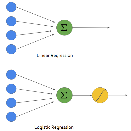
Graphical representation of both linear and logistic regression. The key difference is the application of the squashing function shown in yellow. Original Source - Towards Data Science

To make this intuition concrete, we define each $\hat{f}$ as having the following form (note: this equation looks daunting. We have some tips for interpreting it below).

\[ \begin{aligned} \hat{f}(\mathbf{x}) &= \text{probability that output, $y$, is 1} \nonumber \\ &=\frac{1}{1 + e^{-\mathbf{w}^\top \mathbf{x}}} \tag{2} \end{aligned} \]

Here are a few things to notice about this equation:

1. The weight vector that we saw in linear regression, $\mathbf{w}$, has made a comeback. We are using the dot product between $\mathbf{x}$ and $\mathbf{w}$ (which creates a weighted sum of the $x_i$’s), just as we did in linear regression!
2. As indicated in Figure 1, the dot product $\mathbf{w}^\top \mathbf{x}$ has been passed through a squashing function known as the sigmoid function. The graph of $\sigma(u) = \frac{1}{1+e^{-u}}$ is shown in Figure 2. $\sigma( \mathbf{w}^\top \mathbf{x})$ is exactly what we have in \(\hat{f}(\mathbf{x}) =\frac{1}{1 + e^{-\mathbf{w}^\top \mathbf{x}}}\)

Figure 2:

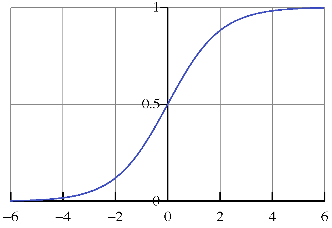
A graph of the sigmoid function $\frac{1}{1+e^{-x}}$.

Deriving the Logistic Regression Learning Rule

Now we will formalize the logistic regression problem and derive a learning rule to solve it (i.e., compute the optimal weights). The formalization of logistic regression will combine Equation 2 with the selection of $\ell$ to be log loss (Equation 1). This choice of $\ell$ results in the following objective function (this is a straightforward substitution. there’s nothing too tricky going on here).

\[\begin{aligned} \mathbf{w}^\star &= \argmin_{\mathbf{w}} \sum_{i=1}^n \Big ( - y_i \ln \sigma(\mathbf{w}^\top \mathbf{x_i}) - (1-y_i) \ln (1 - \sigma(\mathbf{w}^\top \mathbf{x_i}) ) \Big) \\ &= \argmin_{\mathbf{w}} \sum_{i=1}^n \Bigg ( - y_i \ln \left ( \frac{1}{1+e^{-\mathbf{w}^\top \mathbf{x_i}}} \right) - (1-y_i) \ln \left (1 - \frac{1}{1+e^{-\mathbf{w}^\top \mathbf{x_i}}} \right ) \Bigg) &\text{expanded out if you prefer this form} \end{aligned}\]

While this looks a bit intense, since $y_i$ is either 0 or 1, the multiplication of the expressions in the summation by either $y_i$ or $1-y_i$ are essentially acting like a switch—depending on the value of $y_i$ we either get one term or the other. Our typical recipe for finding $\mathbf{w}^\star$ has been to take the gradient of the expression inside the $\arg\,min\,$, set it to $0$, and solve for $\mathbf{w}^\star$ (which will be a critical point and hopefully a minimum). The last two steps will be a bit different for reasons that will become clear soon, but we will need to find the gradient. We will focus on finding the gradient in the next couple of parts.

Useful Properties of the Sigmoid Function

The equation for $\mathbf{w}^\star$ above looks really hairy! We see that in order to compute the gradient we will have to compute the gradient of $\mathbf{x}^\top \mathbf{w}$ with respect to $\mathbf{w}$ (we just wrapped our minds around this last assignment). Additionally, we will have to take into account how the application of the sigmoid function and the log function changes this gradient. In this section we’ll learn some properties for manipulating the sigmoid function and computing its derivative.

Exercise 1

The sigmoid function, $\sigma$, is defined as

\[\begin{align*} \sigma(x) &= \frac{1}{1+e^{-x}} \end{align*}\]

Part A

Show that $\sigma(-x) = 1 - \sigma(x)$.

Solution

\[\begin{align*} \sigma(-x) &= \frac{1}{1+e^{x}} \\ &= \frac{e^{-x}}{e^{-x} + 1}~~\text{multiply top and bottom by $e^{-x}$} \\ \sigma(-x) - 1&= \ \frac{e^{-x}}{e^{-x} + 1} - \frac{1 + e^{-x}}{1 + e^{-x}} ~~\text{subtract $-1$ on both sides} \\ &= \frac{-1}{1+e^{-x}} \\ &= -\sigma(x) \\ \sigma(-x) &= 1 - \sigma(x) \end{align*}\]

Part B

Show that the derivative of the logistic function $\frac{d}{dx} \sigma(x) = \sigma(x) (1 - \sigma(x))$

Solution

Two solutions for the price of 1!

Solution 1:

\[\begin{align*} \frac{d}{dx} \sigma(x) &= e^{-x} \sigma(x)^2 &\text{apply quotient rule} \\ &= \sigma(x) \left ( \frac{e^{-x}}{1 + e^{-x}} \right) &\text{expand out one of the $\sigma(x)$'s}\\ &= \sigma(x) \left ( \frac{1}{e^{x} + 1} \right) & \text{multiply top and bottom by $e^{x}$}\\ &= \sigma(x) ( \sigma(-x)) &\text{substitute for $\sigma(-x)$} \\ &= \sigma(x) (1 - \sigma(x) ) &\text{apply $\sigma(-x)=1-\sigma(x)$} \end{align*}\]

Solution 2:

\[\begin{align*} \frac{d}{dx} \sigma(x) &=\frac{e^{-x}}{(1+e^{-x} )^2} & \text{apply quotient rule} \\ &= \frac{e^{-x}}{1+2e^{-x} + e^{-2x}} & \text{expand the bottom}\\ &= \frac{1}{e^{x}+2 + e^{-x}} & \text{multiply top and bottom by $e^{x}$}\\ &= \frac{1}{(1+e^{x})(1+e^{-x})} & \text{factor} \\ &= \sigma(x)\sigma(-x) & \text{decompose using definition of $\sigma(x)$}\\ &= \sigma(x)(1-\sigma(x)) &\text{apply $\sigma(-x)=1-\sigma(x)$} \end{align*}\]

Chain Rule for Gradients

We now know how to take derivatives of each of the major pieces of the logistic regression loss function. What we need is a way to put these derivatives together. You probably remember that in the case of single variable calculus you have just such a tool. This tool is known as the chain rule. The chain rule tells us how to compute the derivative of the composition of two single variable functions $f$ and $g$.

\[\begin{aligned} h(x)&= g(f(x))&\text{h(x) is the composition of $f$ with $g$} \nonumber \\ h'(x) &= g'(f(x))f'(x)&\text{this is the chain rule!} \end{aligned}\]

Suppose that instead of the input being a scalar $x$, the input is now a vector, $\mathbf{w}$. In this case $h$ takes a vector input and returns a scalar, $f$ takes a vector input and returns a scalar, and $g$ takes a scalar input and returns a scalar.

\[\begin{aligned} h(\mathbf{w}) &= g(f(\mathbf{w}))&\text{h($\mathbf{w}$) is the composition of $f$ with $g$} \nonumber \\ \nabla h(\mathbf{w}) &= g'(f(\mathbf{w})) \nabla f(\mathbf{w}) & \text{this is the multivariable chain rule} \end{aligned}\]

Exercise 2

Part A

Suppose $h(x) = \sin(x^2)$, compute $h’(x)$ (x is a scalar so you can apply the single-variable chain rule).

Solution

Applying the chain rule gives

\[ \begin{aligned} h’(x) &= cos(x^2) 2x \end{aligned} \]

Part B

Define $h(\mathbf{v}) = (\mathbf{c}^\top \mathbf{v})^2$. Compute $\nabla_{\mathbf{v}} h(\mathbf{v})$ (the gradient of the function with respect to $\mathbf{v}$).

Solution

We can see that $h(\mathbf{v}) = g(f(\mathbf{v}))$ with $g(x) = x^2$ and $f(\mathbf{v}) = \mathbf{c}^\top \mathbf{v}$ The gradient can now easily be found by applying the chain rule.

\[ \begin{aligned} \nabla h(\mathbf{v}) &= 2(\mathbf{c}^\top \mathbf{v}) \mathbf{c} \end{aligned} \]

Part C

Compute the gradient of this expression, which comes from the beginning of the section on deriving the logistic regression learning rule:

\[ \begin{aligned} \sum_{i=1}^n -y_i \ln \sigma( \mathbf{w}^\top \mathbf{x_i}) - (1-y_i) \ln \left (1 - \sigma( \mathbf{w}^\top \mathbf{x_i}) \right ) \end{aligned} \]

You can either use the chain rule and the identities you learned about sigmoid, or expand everything out and work from that.

Solution

Applying the chain rule gives us

\[ \begin{aligned} \sum_{i=1}^n -y_i \frac{\nabla \sigma( \mathbf{w}^\top \mathbf{x_i})}{\sigma( \mathbf{w}^\top \mathbf{x_i})} - (1-y_i) \frac{- \nabla \sigma( \mathbf{w}^\top \mathbf{x_i})}{1 - \sigma( \mathbf{w}^\top \mathbf{x_i})} \enspace . \end{aligned} \]

Applying the chain rule again gives us

\[ \begin{aligned} & \sum_{i=1}^n -y_i \frac{\sigma( \mathbf{w}^\top \mathbf{x_i})(1-\sigma( \mathbf{w}^\top \mathbf{x_i}))\nabla \mathbf{w}^\top \mathbf{x_i}}{\sigma( \mathbf{w}^\top \mathbf{x_i})} - (1-y_i) \frac{- \sigma( \mathbf{w}^\top \mathbf{x_i})(1-\sigma( \mathbf{w}^\top \mathbf{x_i}))\nabla \mathbf{w}^\top \mathbf{x_i}}{1 - \sigma( \mathbf{w}^\top \mathbf{x_i})} \nonumber \\ &= \sum_{i=1}^n -y_i (1-\sigma( \mathbf{w}^\top \mathbf{x_i}))\mathbf{x_i} + (1-y_i) \sigma( \mathbf{w}^\top \mathbf{x_i})) \mathbf{x_i} \end{aligned} \]

You could certainly stop here, but if you plug in $y=0$ and $y=1$ you’ll find that the expression can be further simplified to:

\[ \begin{aligned} \sum_{i=1}^n -(y_i - \sigma(\mathbf{w}^\top \mathbf{x_i})) \mathbf{x_i} \nonumber \end{aligned} \]

Gradient Descent for Optimization

If we were to follow our derivation of linear regression we would set our expression for the gradient to 0 and solve for $\mathbf{w}$. It turns out this equation will be difficult to solve due to the $\sigma$ function. Instead, we can use an iterative approach where we start with some initial value for $\mathbf{w}$ (we’ll call the initial value $\mathbf{w^0}$, where the superscript corresponds to the iteration number) and iteratively adjust it by moving down the gradient (the gradient represents the direction of fastest increase for our function, therefore, moving along the negative gradient is the direction where the loss is decreasing the fastest).

External Resources

There are tons of great resources that explain gradient descent with both math and compelling visuals.

• Recommended: Gradient descent, how neural networks learn - Deep learning, chapter 2, start at 5:20
• An Introduction to Gradient Descent
• The Wikipedia page on Gradient Descent
• Ahmet Sacan’s video on gradient descent (this one has some extra stuff, but it’s pretty clearly explained).
• There are quite a few resources out there, do you have some suggestions? (Share on Slack!)

Exercise 3

To test your understanding of these resources, here are a few diagnostic questions.

Part A

When minimizing a function with gradient descent, which direction should you step along in order to arrive at the next value for your parameters?

Solution

The negative gradient (since we are minimizing)

Part B

What is the learning rate and what role does it serve in gradient descent?

Solution

The learning rate controls the size of the step that you take along the negative gradient.

Part C

How do you know when an optimization performed using gradient descent has converged?

Solution

There are a few options. One popular one is to check if the objective function is changing only a minimal amount each iteration, the algorithm has converged. You could also look at the magnitude of the gradient (which tells us the slope) to see if it is really small.

Part D

True or false: provided you tune the learning rate properly, gradient descent guarantees that you will find the global minimum of a function.

Solution

False, the best gradient descent can do, in general, is converge to a local minimum. If you know that the function you are optimizing has only one minimum, then this would also be the global minimum (this is the case for both linear and logistic regression).

If we take the logic of gradient descent and apply it to the logistic regression problem, we arrive at the following learning rule. Given some initial weights $\mathbf{w^0}$, and a learning rate $\eta$, we can iteratively update our weights using the formula below.

We start by applying the results from our exercise on the chain rule.

\[\begin{aligned} \mathbf{w^{n+1}} &= \mathbf{w^n} - \eta \sum_{i=1}^n -(y_i - \sigma(\mathbf{w}^\top \mathbf{x_i})) \mathbf{x_i} \\ &= \mathbf{w^n} + \eta \sum_{i=1}^n (y_i - \sigma(\mathbf{w}^\top \mathbf{x_i})) \mathbf{x_i} ~~~\text{distribute the negative} \end{aligned}\]

This beautiful equation turns out to be the recipe for logistic regression.

Notice

We won’t be assigning a full implementation of logistic regression from scratch. In future assignments, we will spend more time applying logistic regression and gradient descent.

If it’s helpful for your learning to see a worked example with code now (to help the math make sense), you can optionally check out this example of binary classification for admission to college, noting that some of the math notation is slightly different than ours.

You are also welcome to implement logistic regression using gradient descent if it’s helpful for your learning and/or if you already have significant experience with machine learning and want a challenge. This is completely optional, and we assume that most of you will not choose to do this. If you do decide to implement logistic regression using gradient descent, you will need to search for a good learning rate or you may consider implementing some strategies for automatically tuning the learning rate.

Dataflow Diagrams and Foundations of Micrograd

Now that we have derived a learning rule for logistic regression, we are going to look at another way of representing multivariable functions and computing their partial derivatives. This way of thinking about multivariable functions may seem a little strange at first, but this notion is going to lay the foundation for being able to derive learning rules for a whole range of machine learning models in an automated fashion!!

First, let’s look at a multivariable function defined by the equations below. We have a single scalar input variable $t$ that affects both input arguments of $f$ (through $x(t)$ and $y(t)$).

\[\begin{aligned} x &= x(t) \\ y &= y(t) \\ f &= f(x, y) \\ \end{aligned}\]

Let’s represent this system of equations using a data flow diagram (in some resources this is called a tree diagram, in which case it is drawn a bit differently).

flowchart BT id1["$$f = f(x,y)~~~~$$"] id2["$$x = x(t)~~$$"] id3["$$y = y(t)~~$$"] id2 --> id1 id3 --> id1 t --> id2 t --> id3

This diagram represents how data moves from the inputs of a function (in this case $x$ and $y$) to its output (in this case $f$). If we were to take a chart like this and figure out how to evaluate a function given some inputs, you’d have to make sure you always evaluate the inputs to a block before you try to evaluate the block itself. For instance, I wouldn’t be able to evaluate the block $f = f(x,y)$ until I’ve evaluated the blocks $x = x(t)$ and $y=y(t)$. To evaluate a block, you can imagine that the output of a block flows along the arrow into the downstream block, which then processes that input further until it arrives at the output.

Let’s say we want to calculate $\frac{\partial f}{\partial t}$. We’ve learned about the chain rule for single variable functions, but this case is a bit different. It turns out that, in this case, we can compute the partial derivative we seek in the following way.

\[\begin{aligned} \frac{\partial f}{\partial t} &= \frac{\partial f}{\partial x} \frac{\partial x}{\partial t} + \frac{\partial f}{\partial y} \frac{\partial y}{\partial t} \end{aligned}\]

What is this formula saying??? Well it looks awfully like the single variable chain rule in the sense that we are multiplying derivatives together. The only difference is that we are having to account for the multiple pathways from the input (independent variable) $t$ to the output (dependent variable) $f$.

In the resources below, you will see how we can use our data flow diagram to compute these partial derivatives.

External Resources

This Harvey Mudd College calculus tutorials explain the concept of the chain rule using dataflow diagrams. You can view this at HMC Multivariable Chain Rule Page.

There is another nice writeup on this at Math LibreTexts (Note: that this writeup uses a slightly different graph structure where inputs that branch to multiple downstream functions are replicated)

Exercise 4

Draw a dataflow diagram to represent the function $f(x,y,z) = \cos(x^2 y) + x^2 \sqrt{z}$. Compute $\frac{\partial f}{\partial x}, \frac{\partial f}{\partial y}, \frac{\partial f}{\partial z}$ using the dataflow diagram method.

Solution

flowchart BT id1["$$f = h_3 + h_5~~$$"] id2["$$h_3 = \cos(h_2)~~$$"] id3["$$h_5 = h_1 \times h_4~~$$"] id4["$$h_1 = x^2$$"] id5["$$h_4 = \sqrt{z}~~$$"] id6["$$h_2 = h_1 \times y~~$$"] id2 --> id1 id3 --> id1 id4 --> id3 id6 --> id2 id5 --> id3 id4 --> id6 x --> id4 y --> id6 z --> id5

\[ \begin{aligned} \frac{\partial f}{\partial x}&= \frac{\partial h_1}{\partial x} \frac{\partial h_2}{\partial h_1} \frac{\partial h_3}{\partial h_2} \frac{\partial h_f}{\partial h_3} + \frac{\partial h_1}{\partial x} \frac{\partial h_5}{\partial h_1} \frac{\partial f}{\partial h_5} \nonumber \\ &= 2x \times y \times -\sin(h_2) \times 1 + 2x \times h_4 \times 1 \\ &= -2xy \sin(x^2 y) + 2x \sqrt{z} \\ \frac{\partial f}{\partial y} &= \frac{\partial h_2}{\partial y} \frac{\partial h_3}{\partial h_2} \frac{\partial f}{\partial h_3}\nonumber \\ &= h_1 \times -\sin(h_2) \times 1 \\ &= -x^2 \sin(x^2 y) \\ \frac{\partial f}{\partial z} &= \frac{\partial h_4}{\partial z} \frac{\partial h_5}{\partial h_4} \frac{\partial f}{\partial h_5} \\ &= \frac{1}{2} \frac{1}{\sqrt{z}} \times h_1 \times 1 \\ &= \frac{1}{2} \frac{x^2}{\sqrt{z}} \end{aligned} \]

Exercise 5

Come up with your own multivariable function and use a dataflow diagram to compute the partial derivative of the function with respect to each of its inputs. If doable, sanity check your result by computing derivatives by hand.

Solution

This is person-dependent, so no solution here. If you have a nice sample, let us know.

Exercise 6

Suppose we have a logistic regression model with two inputs $x_1$ and $x_2$ (each of these are just scalars now) and binary outputs $y$. Given the data flow diagram for computing the log loss of this logistic regression model, compute the partial derivative of the log loss with respect to each of its weights $w_1$ and $w_2$.

flowchart BT x1["$$x_1$$"] x2["$$x_2$$"] w1["$$w_1$$"] w2["$$w_2$$"] h3["$$h_3 = h_1 + h_2$$"] h1["$$h_1 = x_1 w_1$$"] h2["$$h_2 = x_2 w_2$$"] h4["$$h_4 = \sigma(h_3)$$"] h5["$$\ell = -y\,\ln(h_4) - (1-y)\,\ln(1-h_4)~~~~$$"] x1 --> h1 w1 --> h1 x2 --> h2 w2 --> h2 h1 --> h3 h2 --> h3 h3 --> h4 h4 --> h5 y --> h5

Solution

\[ \begin{aligned} \frac{\partial{\ell}}{w_1} &= \frac{\partial h_1}{\partial w_1} \frac{\partial h_3}{\partial h_1} \frac{\partial h_4}{\partial h_3} \frac{\partial \ell}{\partial h_4} \\ &= x_1 \times 1 \times \sigma(h_3) (1-\sigma(h_3)) \times \Bigg(-y \frac{1}{\sigma(h_3)} + (1-y)\frac{1}{1-\sigma(h_3)}\Bigg) \\ &= - y x_1 \sigma(h_3) (1-\sigma(h_3)) \frac{1}{\sigma(h_3)} + (1-y) x_1 \sigma(h_3) (1-\sigma(h_3)) \frac{1}{1-\sigma(h_3)} \\ &= -y x_1 (1-\sigma(h_3)) + (1-y) x_1 \sigma(h_3) \\ &= - x_1 (y-\sigma(h_3))~~~~~\text{If you plug in $y=0$ and $y=1$ you will see this is true} \\ &= - x_1 (y-\sigma(w_1 x_1 + w_2 x_2)) \end{aligned} \]